1.4.3.2 Junior Debt Spread

🏦 Private infrastructure loan valuation

Private infrastructure loans do not trade on a public market, so observable prices and spreads are scarce. The credit spread of each instrument is therefore modelled rather than read off a screen.

⚙️ Spread modelling and Kalman filter

The model expresses a borrower's credit spread as a combination of its observable risk characteristics, the more risk a lender bears, the wider the spread it demands. Rather than fixing this relationship once, the model updates it continuously with a Kalman filter, so the weight placed on each risk factor adapts as market conditions change. Crucially, each date's estimate uses only information available up to that date, the filter is one sided, with no look ahead, which makes the historical series reproducible and free of hindsight.

📈 Valuation application

The modelled spread then flows into valuation: each instrument's contractual cashflows are discounted on a risk free curve plus its credit spread. The same model is applied consistently across the eligible universe, so that valuations differ only where the data justifies, reflecting each instrument's subordination and its own risk profile.

⚙️ The variables and their impact

Each risk factor enters the spread through an economically interpretable channel. Together they capture the credit, structural and market drivers of what a lender charges.

Probability of default

Credit risk

Sourced from the companion infrastructure credit risk model, it anchors the spread to the borrower's fundamental likelihood of default, the primary measure of credit quality in the framework.

⌛ Maturity

Term structure

The remaining life of the instrument. Maturity is one of the model's most influential factors, shaping how the spread varies across the term structure of a borrower's debt.

💸 Benchmark rate

Rate environment

The prevailing reference interest rate. It lets the credit spread respond to the wider rate environment rather than being modelled in isolation from it.

🏗️ Facility size

Liquidity & scale

Face value of the facility, a proxy for the borrower's scale and the relative liquidity of the exposure.

🏭 Sector

Common factor

The industrial sector: Power, Roads, Social Infrastructure, Renewables and Rail. Sector acts as a systematic common factor. Borrowers in the same sector tend to move together, and different sectors sit at different spread levels. This shared movement is what survives when spreads are aggregated across many borrowers. These sectors are selected because each has enough constituents in the junior universe to estimate a stable, statistically significant loading. Sparse sectors, or those dominated by a single outlier borrower, are folded into a common baseline rather than given their own factor, so every sector effect stays well supported by data.

💰 Business model

Revenue certainty

Whether revenue is contracted or merchant (market exposed). Merchant exposure introduces more cashflow uncertainty, which the market prices as a wider spread.

🛡️ Robustness of the model

Because prices for these instruments are not continuously observable, the framework is validated on the properties that matter for a fundamentally valued asset class: the economic soundness of its factors, the statistical behaviour of the estimates, and the discipline of the data and process behind them.

💸 Economic soundness

📊 Statistical behaviour

🗂 Data & process

📋 Diagnostics from the production model run (2026-07-31)

📊 Model residual distribution

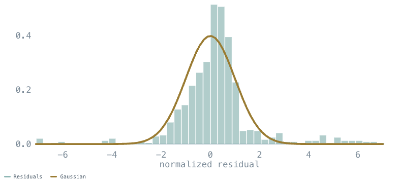
Pricing error summary

The calibration report's histogram of model residuals, reproduced here: each residual is modelled less observed, divided by the model's own standard deviation, shown across three standard deviations against a standard normal. The table expresses the same residuals as a pricing error, in percent of the observed spread (modelled less observed), across the full estimation set, excluding a small number of near zero observed spreads that would distort the percentage. The residuals are centred but heavier tailed than the normal, reflecting the sparse and noisy observation of private junior spreads.

📖 Valuation framework

Scope of the framework. This is a fundamental valuation model for instruments without continuous observable prices. Its purpose is to produce a stable, economically grounded spread and a consistent cross sectional ordering of risk, not to reproduce the moment to moment spread of any single loan. Valuations are model estimates and should be interpreted as such.

📈 Backtesting

Because the Kalman filter is one sided, each date's modelled spread uses only information available up to that date. The historical series is therefore an out of sample record, reproducible and free of hindsight.

Each cycle the specification is chosen against competing specifications on out of sample error, and this specification is the selected model. Following the model selection report's actual against model check, the chart compares the actual spread with the modelled spread from 2020 onward for the junior universe, as the annual average, with the final two years held out of sample.

📊 Modelled spread vs. observed, mean

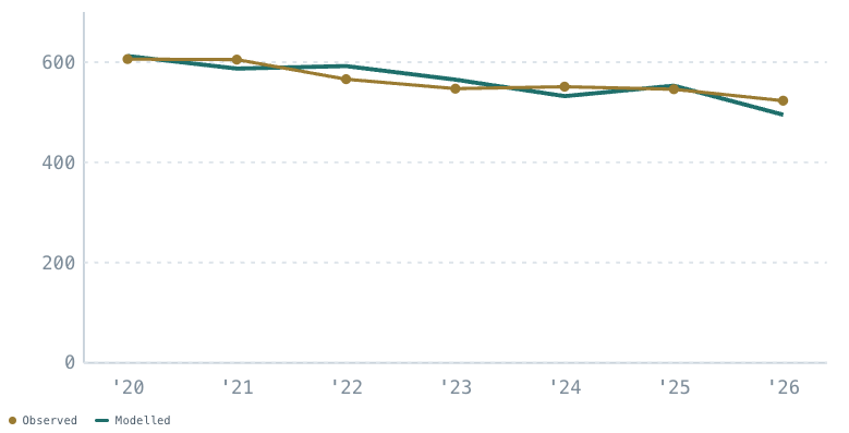
Annual average of the actual and modelled spread, averaged in the model's log space as in the model selection report, using all observations. The model and the actual track closely across this period. Spreads in basis points.